Mock traces example
[1]:
import os
import sys
from radiocalibrationtoolkit import *
[INFO] LFmap: Import successful.
[2]:
piko = 1e-12
[3]:
# some global plot settings
plt.rcParams["axes.labelweight"] = "bold"
plt.rcParams["font.weight"] = "bold"
plt.rcParams["font.size"] = 16
plt.rcParams["legend.fontsize"] = 12

plt.rcParams["xtick.major.width"] = 2
plt.rcParams["ytick.major.width"] = 2

plt.rcParams["xtick.major.size"] = 5
plt.rcParams["ytick.major.size"] = 5

plt.rcParams["xtick.labelsize"] = 14
plt.rcParams["ytick.labelsize"] = 14
[4]:
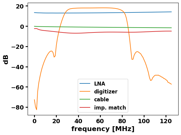
# read HW response
hw_file_path = "./antenna_setup_files/HardwareProfileList_realistic.xml"
hw_dict = read_hw_file(hw_file_path, interp_args={"fill_value": "extrapolate"})
hw_reponse_1 = hw_dict["RResponse"]["LNA"]
hw_reponse_2 = hw_dict["RResponse"]["digitizer"]
hw_reponse_3 = hw_dict["RResponse"]["cable_fromLNA2digitizer"]
hw_reponse_4 = hw_dict["RResponse"]["impedance_matching_EW"]
# merge all hw responses to one function
def hw_response_func(x):
return dB2PowerAmp(
hw_reponse_1(x) + hw_reponse_2(x) + hw_reponse_3(x) + hw_reponse_4(x)
)
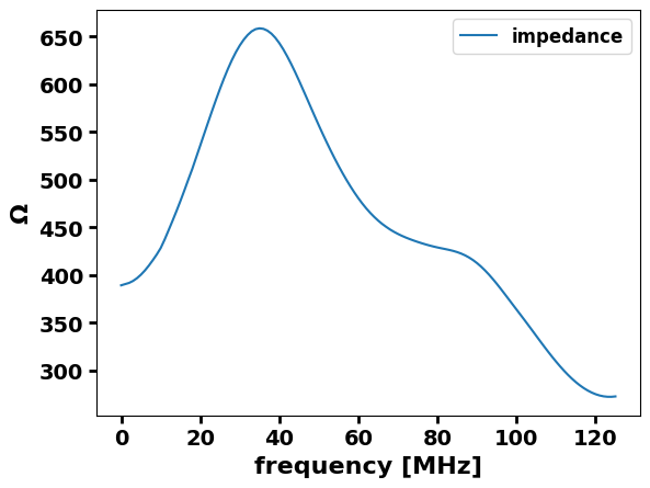
# impedance function
impedance_func = hw_dict["IImpedance"][
"antenna_EW"
]
# read sidereal voltage square spectral density
sidereal_voltage2_density_DF = pd.read_csv(
"./voltage2_density/voltage2_density_Salla_EW_GSM16.csv",
index_col=0,
)
sidereal_voltage2_density_DF.columns = sidereal_voltage2_density_DF.columns.astype(
float
)
<?xml version="1.0" encoding="iso-8859-1"?>
<Element HardwareProfileList at 0x7ff0db7612c0>
[5]:
fig, ax = plt.subplots()
frequencies = np.linspace(0,125,126)
ax.plot(frequencies, hw_reponse_1(frequencies), label='LNA')
ax.plot(frequencies, hw_reponse_2(frequencies), label='digitizer')
ax.plot(frequencies, hw_reponse_3(frequencies), label='cable')
ax.plot(frequencies, hw_reponse_4(frequencies), label='imp. match')
ax.set_xlabel('frequency [MHz]')
ax.set_ylabel('dB')
ax.legend()
[5]:
<matplotlib.legend.Legend at 0x7ff0db7e6320>
[6]:
fig, ax = plt.subplots()
frequencies = np.linspace(0,125,126)
ax.plot(frequencies, impedance_func(frequencies), label='impedance')
ax.set_xlabel('frequency [MHz]')
ax.set_ylabel('$\Omega$')
ax.legend()
[6]:
<matplotlib.legend.Legend at 0x7ff152d49cc0>
The power obtained from the spectra calculated by applying the Discrete Fourier Transform (DFT) to time traces is calculated as follows:
\begin{equation} P_s = 2\frac{1}{T} \sum_{k=f}^{f+\delta f} \frac{|X(k)|^2}{R(f)} \Delta f \end{equation}
where \(\Delta t\) is the sampling time, \(T\) the time trace length, \(N\) the number of samples, \(f_s\) sampling frequency and \(R\) the impedance,
where
\begin{equation} X(k) = X(k)_{DFT} \Delta t = \frac{X(k)_{DFT}}{fs} \end{equation}
where \(X(k)_{DFT}\) is “one-sided” absolute spectrum obtained by applying discrete Fourier transform to the time trace.
On the other hand, the power deposited to antenna by the galactic radio emission is calculated as:
\begin{equation} P_{sky}(t,f) = \frac{k_{b}}{c^{2}} \sum_{f} f^{2} \int_{\Omega} T_{sky}(t,f,\theta,\phi) \frac{|H(f,\theta,\phi)|^{2}Z_{0}}{R(f)} \Delta f d\Omega \end{equation}
where \(Z_0\) is the vacuum impedance, \(R_r\) is the antenna impedance, \(k_b\) the Boltzmann constant and \(c\) is the speed of light.
Denoting power spectral density as
\begin{equation} S_{P}(t,f) = \frac{k_{b}}{c^{2}} f^{2} \int_{\Omega} T_{sky}(t,f,\theta,\phi) \frac{|H(f,\theta,\phi)|^{2}Z_{0}}{R(f)} d\Omega \end{equation}
we can rewrite the equation as
\begin{equation} P_{sky}(t,f) = \sum_{f} S_{P}(t,f) \Delta f \end{equation}
Further, the voltage square density \(S_{\nu}(t,f)\) we defined as
\begin{equation} S_{\nu}(t,f) = \frac{S_{P}(t,f)}{R(f)} \end{equation}
or as:
\begin{equation} S_{\nu}(t,f) = U_{\nu}^2 \end{equation}
Equating the two definitions of power yields:
\begin{equation} 2\frac{1}{T} \sum_{k=f}^{f+\delta f} \frac{|X(k)|^2}{R(f)} \Delta f = \frac{k_{b}}{c^{2}} \sum_{f} f^{2} \int_{\Omega} T_{sky}(t,f,\theta,\phi) \frac{|H(f,\theta,\phi)|^{2}Z_{0}}{R_{r}} \Delta f d\Omega \end{equation}
\begin{equation} 2\frac{1}{T} \frac{|X(k)|^2}{R(f)} = \frac{k_{b}}{c^{2}} f^{2} \int_{\Omega} T_{sky}(t,f,\theta,\phi) \frac{|H(f,\theta,\phi)|^{2}Z_{0}}{R(f)} d\Omega \end{equation}
\begin{equation} 2\frac{1}{T} |X(k)|^2 = \frac{k_{b}}{c^{2}} f^{2} Z_{0} \int_{\Omega} T_{sky}(t,f,\theta,\phi) |H(f,\theta,\phi)|^{2} d\Omega \end{equation}
\begin{equation} 2\frac{1}{T} |X(k)|^2 = S_{\nu}(t,f) \end{equation}
\begin{equation} |X(k)|^2 = \frac{1}{2} T S_{\nu}(t,f) \end{equation}
\begin{equation} |X(k)_{DFT}|^2 \Delta t^2 = \frac{1}{2} T S_{\nu}(t,f) \end{equation}
\begin{equation} |X(k)_{DFT}|^2 = \frac{T}{\Delta t^2} \frac{1}{2} S_{\nu}(t,f) \end{equation}
\begin{equation} |X(k)_{DFT}|^2 = \frac{N f_{s}^2}{ f_s} \frac{1}{2} S_{\nu}(t,f) \end{equation}
\begin{equation} |X(k)_{DFT}|^2 = \frac{N f_{s}}{2} S_{\nu}(t,f) \end{equation}
\begin{equation} |X(k)_{DFT}| = \sqrt{\frac{N f_{s} }{2}} \sqrt{S_{\nu}(t,f)} \end{equation}
A small reminder of the system parameter relations:
\begin{equation} \Delta f = \frac{fs}{N} = \frac{1}{N\Delta t} = \frac{1}{T} \end{equation}
\begin{equation} fs = \frac{1}{\Delta t} \end{equation}
Thermal noise:
\begin{equation} v^2 = 4 k_B T R \end{equation}
where \(k_B\) is the Boltzmann constant, \(T\) is the temperature and \(R\) is the impedance.
source: https://en.wikipedia.org/wiki/Johnson%E2%80%93Nyquist_noise
[7]:
mock_trace_generator = Mock_trace_generator(
    sidereal_voltage2_density_DF=sidereal_voltage2_density_DF,
    hw_response_func=hw_response_func,
    impedance_func=impedance_func,
    voltage2ADC=2048,
    time_trace_size=2048,
    sampling_frequency_MHz=250,
)
freq_MHz_bins = mock_trace_generator.get_frequency_bins()
[8]:
mock_traces_DF = mock_trace_generator.generate_mock_trace(5, nbi = {"67": 1}, nbi_err=0.3)
100%|█████████████████████████████████████████████| 5/5 [00:00<00:00, 31.57it/s]
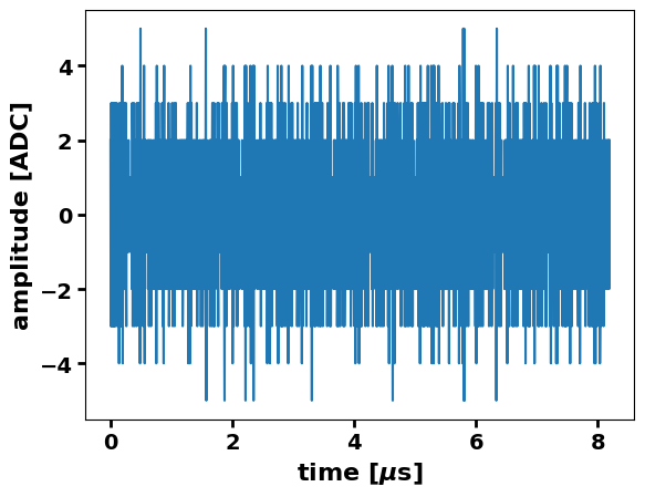
[9]:
fig, ax = plt.subplots()
ax.plot(mock_traces_DF.columns.values[2:], mock_traces_DF.iloc[1,2:])
ax.set_xlabel('time [$\mu$s]')
ax.set_ylabel('amplitude [ADC]')
[9]:
Text(0, 0.5, 'amplitude [ADC]')
[10]:
additional_noise = 5e-4*piko

debug_spectra_dict = mock_trace_generator.generate_mock_trace(
    1, lst=15, temp_celsius=4, nbi={"67": 1}, nbi_err=0.3, return_debug_dict=True, additional_noise=additional_noise
)[0]
100%|████████████████████████████████████████████| 1/1 [00:00<00:00, 295.02it/s]
[11]:
debug_spectra_dict
[11]:
{'freq_MHz_bins': array([0.00000000e+00, 1.22070312e-01, 2.44140625e-01, ...,
        1.24755859e+02, 1.24877930e+02, 1.25000000e+02]),
 'sidereal_voltage2_density': array([-1.23074004e-18, -1.19722424e-18, -1.16370843e-18, ...,
         2.75556423e-18,  2.74667132e-18,  2.73777842e-18]),
 'thermal_noise_voltage2_density': array([5.95840564e-18, 5.96073384e-18, 5.96306205e-18, ...,
        4.17421282e-18, 4.17493029e-18, 4.17564775e-18]),
 'total_voltage2_density_scattered': array([7.02303137e-19, 1.90825834e-18, 9.80767572e-18, ...,
        8.53296068e-18, 6.48329990e-18, 5.42066595e-18]),
 'total_voltage2_density_scattered_in_HW': array([4.51390937e-25, 1.00537884e-24, 4.23567878e-24, ...,
        9.02415837e-23, 6.79555824e-23, 5.63123609e-23]),
 'total_voltage2_density_scattered_in_HW_with_additional_noise': array([1.32079558e-17, 1.45891803e-16, 1.12583452e-15, ...,
        2.20698767e-16, 1.05607496e-15, 9.18125548e-17]),
 'spectrum_voltage_density_in_HW': array([3.39935405e-07, 5.07323353e-07, 1.04131348e-06, ...,
        4.80643791e-06, 4.17092665e-06, 3.79683610e-06]),
 'spectrum_voltage_density_in_HW_with_additional_noise': array([0.00183881, 0.00611133, 0.01697686, ..., 0.00751657, 0.01644248,
        0.00484809]),
 'spectrum_voltage_density_in_HW_with_additional_noise_with_NBI': array([0.00183881, 0.00611133, 0.01697686, ..., 0.00751657, 0.01644248,
        0.00484809]),
 'time_trace': array([-3, -2,  1, ..., -3,  1,  2]),
 'additional_noise': array([3.43998680e-16, 8.49000668e-16, 7.55411496e-17, ...,
        4.24450046e-16, 1.26742860e-15, 2.60854136e-17])}
[12]:
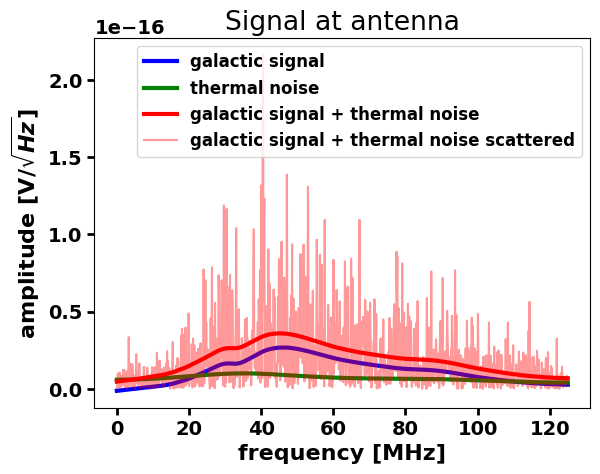
x = debug_spectra_dict["freq_MHz_bins"]
fig, ax = plt.subplots()
ax.set_title("Signal at antenna")
ax.plot(
x,
debug_spectra_dict["sidereal_voltage2_density"],
lw=3,
label="galactic signal",
color="b",
)
ax.plot(
x,
debug_spectra_dict["thermal_noise_voltage2_density"],
lw=3,
label="thermal noise",
color="green",
)
ax.plot(
x,
debug_spectra_dict["sidereal_voltage2_density"]
+ debug_spectra_dict["thermal_noise_voltage2_density"],
label="galactic signal + thermal noise",
lw=3,
color="r",
)
ax.plot(
x,
debug_spectra_dict["total_voltage2_density_scattered"],
alpha=0.4,
label="galactic signal + thermal noise scattered",
color="r",
)
ax.set_xlabel("frequency [MHz]")
ax.set_ylabel("amplitude [V/$\sqrt{Hz}]$")
ax.legend()
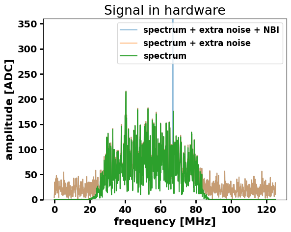
fig, ax = plt.subplots()
ax.set_title("Signal in hardware")
volts2adc = 2048
ax.plot(
x,
debug_spectra_dict["spectrum_voltage_density_in_HW_with_additional_noise_with_NBI"] * volts2adc,
alpha=0.5,
label="spectrum + extra noise + NBI",
)
ax.plot(
x,
debug_spectra_dict["spectrum_voltage_density_in_HW_with_additional_noise"] * volts2adc,
alpha=0.5,
label="spectrum + extra noise",
)
ax.plot(
x,
debug_spectra_dict["spectrum_voltage_density_in_HW"] * volts2adc,
alpha=1,
label="spectrum",
)
ax.set_xlabel("frequency [MHz]")
ax.set_ylabel("amplitude [ADC]")
ax.set_ylim(0, 360)
ax.legend()
[12]:
<matplotlib.legend.Legend at 0x7ff0da7f6590>